Addressing Tail Risk within FRTB

In this paper I want to examine some pivotal concepts that are provided in the risk calculation methodology within the FRTB documentation provided by the Basel Committee on Banking Supervision (BCBS). One of the major purposes in bringing forward the FRTB requirements was for the BCBS to address tail risk in financial markets, a key omission in the Basel II framework. In order to get a better handle on how FRTB is deigned to tackle this task we need to examine and elucidate the specific terminology that the BCBS uses.

The language within BCBS documents describing the FRTB requirements can sometimes be opaque. One of the key terms that is used throughout is “risk factor” and it is important to understand what the BCBS intends with this concept.

A glossary is provided in a Consultative Document on FRTB (https://www.bis.org/publ/bcbs265.pdf) and this includes the following definition:

- Risk factor: A principal determinant of the change in value of a transaction that is used for the quantification of risk. Risk positions are modelled by risk factors.

Since this, in turn, invokes another key term – “risk position” - we should consider that as well:

- Risk position: A risk position is a conceptual construct that represents a particular aspect of risk associated with a transaction within a market risk model or a standardised approach for market risk.

What is emerging from this rather obtuse language is the notion that a risk factor is a modelling tool for quantifying the risk of a specific market exposure.

Perhaps the clearest the BCBS gets to a clear definition of risk factors is to be found when they go on to define a “risk factor class” as follows:

Risk factor class: (Component) Risk factors are mapped to the risk factor classes equity, credit, interest rate, commodities and FX.

Five risk factor classes – or broad categories of risk factors – have been identified and the example that the BCBS document provides for a “risk position” is the closest we can get to a clear understanding of the practical application of risk factors to a market instrument.

Example: A bond denominated in a currency different to a bank’s reporting currency may be mapped to a risk position for FX risk, a number of risk positions for interest rate risk (in the foreign currency) and one or more risk positions for cred it risk.

Finally, we have a reference to something that would actually be found in a bank’s trading book i.e. a bond. This is critical since this is what the actual valuations of trading book positions and the P&L determination, hinge on. For practical purposes, what has emerged is that when evaluating the risk of real world market instruments there is need to map the risk of those instruments to the five different risk factor classes and in determining the overall risk (for regulatory purposes) we need to consider the combined impact of these different types of risk.

What could be behind the rather abstract language that the BCBS has used for risk factors?

Firstly, it ties in neatly with the way that the Basel Committee describes metrics for calculating other metrics. For example, when the BCBS describes the standardized approach for measuring counter party credit risk (SA-CCR can be found in https://www.bis.org/publ/bcbs279.pdf) there is similar reliance on using risk factors.

Secondly, and this is especially relevant to the intent within FRTB, the Committee wants to place the focus on measuring market risk by reference to the availability of high quality and publicly available time series data. To achieve this goal, the focus is being placed on price behaviour at the generic asset class level rather than for the multitude of specific instruments within asset classes where the integrity (and availability) of the time series data can be problematic.

To take an example, let us suppose that a US bank is going to model the market risk for a portfolio of large cap equities with many different company exposures, the relevant primary risk factor for modelling this risk would be US equity and specifically the S&P 500. The bank can then use time series data for this benchmark index as a proxy for its idiosyncratic exposure. Just to point out one advantage here would be to consider the following. Let us suppose that within the bank’s equity portfolio are shares of company XYZ and this company has only been trading for the last two years. Accordingly, there is a shortage of historical price data available. This becomes especially relevant when the bank has to conduct stressed risk analysis (Stressed Expected Shortfall) which is designed to look back for stressful market episodes over a prolonged period. In fact the look-back horizon required under FRTB has to extend back to at least 2007.

The emphasis on availability of extensive historical data is also reflected in one of the most important, and controversial, differentiations within the FRTB framework - the distinction between modellable risk factors and non-modellable risk factors (NMRF’s).

To support the distinction the Basel Committee defines the following:

“Real” prices: A criterion for assessing whether risk factors will be amendable to modelling. A price will be considered “real” if: it is a price from an actual transaction conducted by the bank; it is a price from an actual transaction between other parties (e.g. at an exchange); or it is a price taken from a firm quote (i.e. a price at which the bank could transact).

Furthermore, in order for a risk factor to qualify as modellable there must have been at least 24 observable ‘real’ prices per year, with a maximum of one month between two consecutive observations. Any risk factors that do not meet the criteria would be deemed non-modellable and would have to be capitalised using alternative methods which would result in a substantially higher capital charge. It is precisely, the likelihood that many kinds of exposures found within a bank’s trading book would fall into the bucket of non-modellable risk factors resulting in increased capital requirements, that there has been criticism and push bank from many banks on this distinction.

Another type of criticism, related to the previous discussion, which has been made by several bankers is discussed in an interesting article available from Risk.net. The article entitled “Banks bemoan FRTB model guidance” (available at http://www.numerix.com/risk-magazine-april-2017-special-report-fundamental-review-trading-book) focuses on the notion that FRTB has “left dealers confused on how best to calibrate their internal models”

The following extract from the article pinpoints the concerns about non-modellable risk factors:

The FRTB framework sets out two conflicting ways of generating a desk’s RTPL, however. One version tells a bank to use its back office risk models; the other requires the bank to use its front-office model, but applying only the more limited set of factors that exist in these risk models.... Banks’ front-office models are generally more risk sensitive, incorporating thousands of risk factors to accurately price trading positions. For the RTPL to be a close match, a similar number of risk factors would therefore have to be incorporated into the risk model, making it more granular....

But in order for risk factors to be capitalised under the IMA, they have to meet strict observability criteria. Those that fall short are categorised as non-modellable risk factors (NMRFs) and are capitalised separately, and more punitively....

The tension that is highlighted in this extract is indeed one of the reasons why I thought it worthy to dig as deeply into understanding the rationale and consequences of the Committee’s focus on risk factors and their granularity, or lack thereof.

Let me now move on from some criticisms regarding FRTB to a wider discussion of the way that risk is quantified within the internal models used by banks that are eligible to use the IMA.

EXPECTED SHORTFALL REPLACES VALUE AT RISK

The revised internal models approach (IMA) replaces VaR and stressed VaR with a single Expected Shortfall (ES) metric. ES measures the riskiness of a position by considering both the size and the likelihood of losses above a certain confidence level. This ensures the capture of tail risks that are not accounted for in the existing VaR measures. Expected Shortfall is the expected value (i.e. mean) of the region beyond a specified confidence level.

The Basel Committee does not prescribe a set procedure or model for calculating Expected Shortfall model but makes the following point:

So long as each model used captures all the material risks run by the bank, as confirmed through P&L attribution and back testing…supervisors may permit banks to use models based on either historical simulation, Monte Carlo simulation, or other appropriate analytical methods.

Expected shortfall must be computed on a daily-basis for the bank-wide internal model for regulatory capital purposes. Expected shortfall must also be computed on a daily basis for each trading desk that a bank wishes to include within the scope for the internal models approach for regulatory capital purposes.

For measures based on stressed observations (ESR,S), banks must identify the 12-month period of stress over the observation horizon in which the portfolio experiences the largest loss. The observation horizon for determining the most stressful 12 months must, at a minimum, span back to and include 2007. Observations within this period must be equally weighted. Banks must update their 12-month stressed periods no less than monthly, or whenever there are material changes in the risk factors in the portfolio.

Guidance is provided by the BCBS as to those market conditions which will subject portfolios to stress and banks should provide supervisors with evidence that they have correctly identified those conditions which would have created the largest loss scenarios for the various instruments that are currently found in their trading book.

The current portfolio should be tested against the twelve-month periods surrounding the following events:

• 1987 equity crash
• Exchange Rate Mechanism crises of 1992/3
• Increase in interest rates in Q1, 1994
• 1998 Russian financial crisis
• 2000 bursting of the technology stock bubble
• 2007–08 sub-prime crisis
• 2011–12 Euro zone crisis

Testing should incorporate both large price movements and the sharp reduction in liquidity associated with these events.

To illustrate how the stressed ES method can be used for a specific portfolio let me take as an example a Japanese bank which has current trading book exposure to large-cap Japanese equities. The primary risk factor that would be suitable here would be Japanese equities and the appropriate time series data would come from the Nikkei 225 index.

The first step would be to identify the one-year period which would subject the current portfolio to the maximum stress. Let us suppose that this has been identified as occurring during April 2008 – March 2009. Daily closing price data is obtained for this period and the daily returns are calculated. The ES value for this stress period can then be calculated according to the steps outlined below.

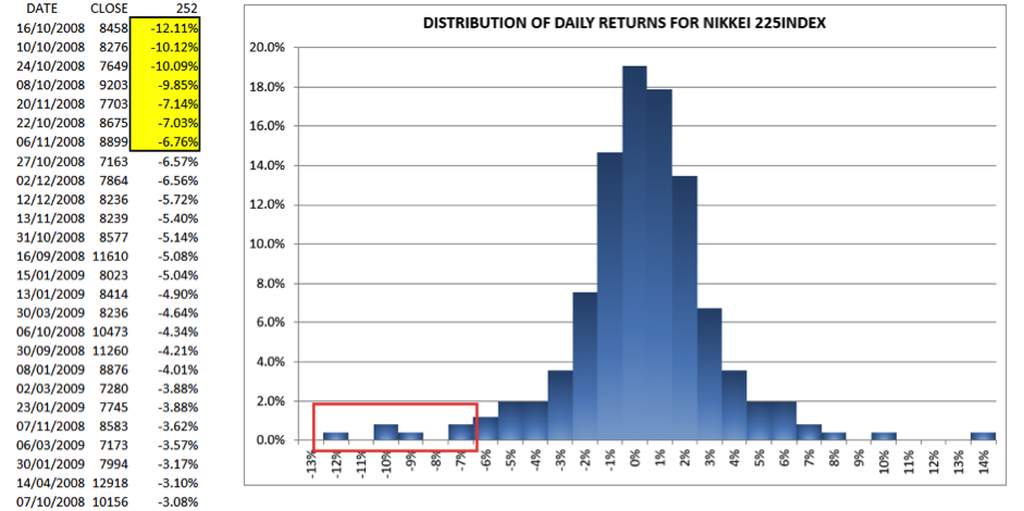
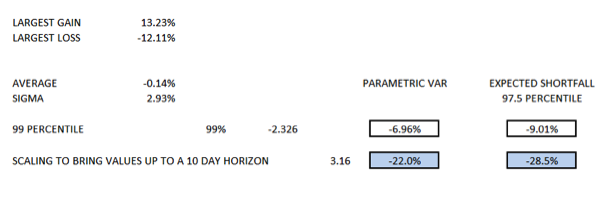
The daily closes and returns have been ranked for all 252 data points (typically this is the number of trading days per year) starting with the largest daily losses at the top. The largest daily gain during the period is shown at 13.23% and the largest daily loss is shown at 12.11%. Worth noting is the daily standard deviation at almost 3% which is about 3 times higher than this value would have during “normal” market conditions.

A frequency distribution has been created positioning each of the daily losses in buckets according to daily percent changes and these are shown in the above histogram. The red rectangle shows the area of the tail that is included in the Expected Shortfall calculation.

Since there are 252 data points, and we need to calculate ES for the 97.5% confidence level, the tail consists of 2.5% of 252 data points which needs to be rounded up to seven days. To determine the Expected Shortfall metric we should average the returns for the worst seven days (as highlighted in the graphic). The ES value is just over 9%. However, this is based on daily returns and the FRTB requirement is that the value has to be calculated using a ten-day horizon. We can scale the ES – using the square root of time rule – by the square root of ten to find the FRTB required value which is 9.01% multiplied by 3.16 or 28.5%

It is also interesting to compare this value with the 10-day parametric VaR value calculated at the 99% confidence level (CI) which is 22%. Again, this has been scaled up from the one-day value which is found by multiplying the standard deviation by -2.33 (i.e. the standard normal deviate for this CI level on a one tailed distribution) and adding this to the mean return.

It is apparent from the histogram that the time series data is not normally distributed and has a long left-tail and this has been captured by the fact that the 10-day ES value is more than six percent higher than the 10 day parametric VaR value.

From this simplified analysis we can determine that the Stressed ES value required for FRTB purposes for the bank’s portfolio of large cap Japanese equities should assume a 28.5% shock to the portfolio. The actual ES calculation can be refined by using a ten day overlay or segmentation of the underlying time series data, such that a ten-day average and a ten day sigma value are calculated and then the resulting values do not require scaling with the square root of time short-cut.

LIQUIDITY HORIZONS

An innovative approach to the market risk capital charge has been introduced under FRTB which relates to the need to factor market liquidity into the calculations. The Committee wanted to address concerns that the pre-FRTB Basel III framework for market risk used a 99% VAR over a standard ten-day horizon. This assumes that market conditions will always be sufficient for a bank to liquidate outstanding positions over this horizon. The 2007/8 crisis provide plenty of examples which contravened this assumption. Moreover, the one-size-fits- all approach does not account for differing levels of liquidity for various products. Put simply, it can significantly underestimate the difficulty of exiting complex and illiquid assets. This is also in accordance with IFRS 13 standards and methods for fair market valuation which hinge on determining an exit price for disposing of assets which must take into account both the type of financial instrument as well as overall market liquidity conditions.

Under FRTB, the default liquidity horizon for the ES metric remains at 10 days but horizons range from 10 to 120 days depending on the risk factor (s), or to paraphrase from our earlier discussion it hinges on the specific characteristics and complexity of the asset type.

Let us take a simple example where the primary risk factor is FX. For foreign exchange positions in the major specified currencies, i.e. EUR, USD, GBP, JPY, CAD, SEK, AUD and the domestic currency of a bank - the ES value would correspond to the standard 10-day horizon.

For unspecified or minor currencies the liquidity horizon has been set at 20 days. Since, as previously discussed, volatility scales according to the square root of time, the ES value for a position in a minor currency must be scaled by the square root of 20/10 = 1.43. Credit spread volatility products require the application of a 120-day horizon, so the scaling of the ES would be the square root 120/10 which is equal to 3.46.

The focus of this discussion has been on the Basel Committee’s expressed intent to rectify the shortcomings of previous methods for calculating outlier risks that are always present within a bank’s trading book. The FRTB framework in many respects is very complex and has been subjected to a considerable amount of criticism from practitioners in the banking world. The core elements of Expected Shortfall and graduated liquidity horizons for different asset types (risk factors) are significant steps forward in what is the most challenging area of financial risk – the measurement and management of tail risk.

About the Author

Clive Corcoran

Clive Corcoran has been engaged in the finance and investment management sectors, on both sides of the Atlantic, for more than 25 years. After completing his education in the UK, Canada and the US, he co-founded and became the CEO of an investment management company based in the USA during the 1980’s and 90’s. The company provided wealth management and fiduciary services to a variety of international clients.

Since re-locating to the UK in 2000, he has continued, as an FCA registered investment adviser, to be engaged in providing strategic investment advice to private clients and pension funds. During recent years he has written several books on international finance, focusing on asset allocation and risk management. He also has also been very actively involved in executive education on a global basis for finance professionals. He conducts workshops and in house courses on a variety of topics including risk management, Basel III and capital adequacy, central banking, systemic risk, asset allocation techniques, credit risk, market risk and derivatives.

Some of the clients for whom he has provided in house training include the European Central Bank in Frankfurt, a central bank in the Eurozone, three of Europe’s G-SIB banks, the largest bank in Russia, one of China’s G-SIB banks, a central bank in North Africa, a sovereign wealth fund in the Gulf, China’s largest asset management company in Beijing, commercial banks in sub-Saharan Africa, a global banking group domiciled in the Netherlands, a central bank in South America, a public/private partnership in project finance based in Washington D.C., a major European clearing organization and the European Investment Bank (EIB).